Posted by Armin on Saturday, February 26, 2011
Thanks to Kevin Ford and Janneke Hille Ris Lambers at UW I recently had the opportunity to get access to a very good-looking LIDAR data set for the area around Mount Rainier, WA. They obtained a high-resolution LIDAR map of Mt. Rainier National Park from the Puget Sound Lidar Consortium. Kevin and Janneke approached me to ask whether it's possible to create a 3D print of Mount Rainier and, naturally, I was extremely intrigued by this idea.
The data Kevin gave me covered a bit more than 30 by 30 km with circa 10 million elevation samples. This incredibly high resolution made the map look incredibly beautiful in GIS software, but it also presented a substantial problem for me. In order to create anything printable, I had to drastically down-sample the data points. Another problem was that the elevation data behaves like a 2D sheet floating in 3D space, but in order to print something on a 3D printer, I needed nodes that describe a closed 3D volume. The project therefore involved a fair bit of data manipulation, which I describe below.
Getting Mount Rainier into Matlab and Meshlab
Getting the data into Matlab was a bit of a challenge because our lab computer wasn't quite prepared for the 10-million point map data. I decided to use Meshlab to downsample the model, so that I was left with only about 100,000 points. At this point, another complication arose: Meshlab couldn't read the Shapefile format file I received. In order to read the data file into Meshlab, I had to convert the original one into a [X,Y,Z] - type ASCII file. To save memory, I used Matlab's textscan function to read in the original in chunks, and then append the [X,Y,Z] coordinates to a new file.
Code to convert large 4-column ASCII data file into 3-column ASCII file
Once I had the data in a format (.asc) that Meshlab could read, I used the Poisson disk sampling filter to subsample the data cloud. Now, the data could be loaded back into Matlab, and it looks as follows:

The red box is the region I decided to use for the printed 3D model.
Creating a base for the mountain to stand on
The next step was to find the points at the edges of the square box shown in the figure above. Then, I looped through each of these points to create a vertical "curtain" of 3D points along the edges down to a base, which I set at sea level. Finally, to achieve a point cloud that describes a closed volume, I put a horizontal plate of points at sea level underneath the mountain. After this step is done, the point cloud now has about 430,000 particles and looks like the following image (edges indicated by red markers, now looking down from the north):

The point cloud gets triangles that describe surface mesh
The 3D printer accepts STL files, which describe an object as 3-dimensional nodes and triangles (faces) that connect the nodes. The faces ned to be arranged so they tile the outside of the volume. Luckily for me, there are a handful of very convenient tools out there for doing this kind of surface reconstruction.
I used the "crust algorithm" implemented by Luigi Giaccari, which takes a dense 3D scatter cloud as an input, and returns a tight, manifold triangulation. (http://www.advancedmcode.org/surface-recostruction-from-scattered-points...)
Now the mountain has a 3D triangular mesh associated with it. Yay! Just to be sure there were no mistakes in the mesh, I ran it through another very useful function found in the iso2mesh toolbox by Qianqian Fang (http://iso2mesh.sf.net):
Now the mesh was ready to be re-imported into Meshlab. Again, I used tools from the fabulous iso2mesh toolbox to save the data in some common formats, such as VRML or OFF:
Back in Meshlab to check out the mesh and export as STL
In addition to including many very useful filters for 3D surface reconstruction, Meshlab (http://meshlab.sourceforge.net/) renders even a huge mesh impressively fast and in a beautiful fashion. It also allowed me to save the mesh in STL format, which our printer software understands.

Printing it in 3D
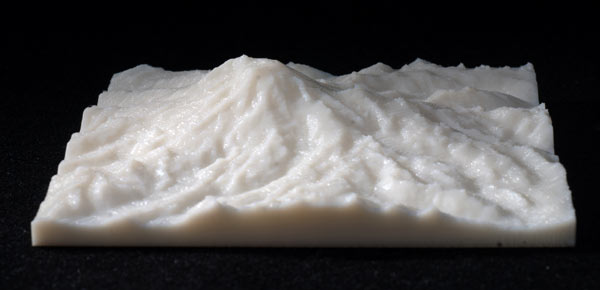
The STL of the mesh shown above was used to print a model of the mountain with a 5x5 inch (12.7x12.7 cm) footprint on the Daniel Lab's uPrint 3D printer. Since each edge corresponds to about 26.5 km in the real world, we now have ca. 4.8 mm of model for one kilometer in real life. Since Mount Rainier's summit elevation is 4392 m, the model comes out to be 21.1 mm tall.
 Printout scale 1:208661
I've also printed a second model in which I zoomed in a bit more. The base is now 20x20 kilometers, which gives us ca. 6.3 mm of model for one real-world kilometer. The mountain is now about 27.7 mm high.
 Printout scale 1:157480
Time-lapse video of the print process
Rapid prototyping is fast compared to traditional machining techniques, but it's not all that rapid either. Printing the mountain took about 6 hours. An iSight camera placed in front of the printer shows the process condensed into a short movie:
Data source
Mount Rainier National Park Bare Earth LiDAR DEM [computer file]. Available: Puget Sound LiDAR Consortium, Seattle, WA http://pugetsoundlidar.ess.washington.edu/index.htm [February 2011].